Rolling Beta, Self-Weight Bias, and a Leave-One-Out Fix
The question
Beta is the standard measure of how much a stock moves relative to a benchmark:
\[\beta_t = \frac{\text{Cov}(R_{i,t}, R_{bench,t})}{\text{Var}(R_{bench,t})}\]
computed over a trailing window so it can be tracked over time rather than collapsed into one number for all history. A rolling beta immediately shows something a static beta hides: the relationship between a stock and its benchmark drifts, sometimes a lot.
def rolling_beta(asset_ret, bench_ret, window=60):
    cov = asset_ret.rolling(window).cov(bench_ret)
    var = bench_ret.rolling(window).var()
    return cov / var
Below is AAPL’s rolling beta to SPY over roughly a decade, computed at two window lengths. The dashed line marks beta = 1 (moving exactly like the index).
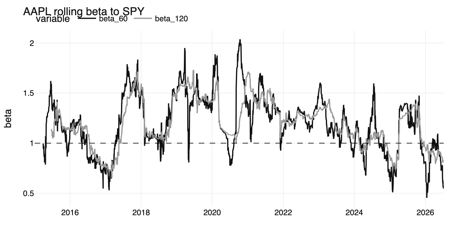
The 60-day line reacts faster and is noisier; the 120-day line is smoother but lags. That’s the standard bias–variance trade-off of any rolling window, wearing a time-series costume.
A question worth asking: does index weight inflate beta?
Here’s a subtlety that’s easy to miss. For a cap-weighted index, the index return is literally a weighted sum of its constituents:
\[R_{index} = \sum_i w_i R_i\]
Substituting that into the covariance in the beta formula:
\[\text{Cov}(R_i, R_{index}) = w_i \cdot \text{Var}(R_i) + \sum_{j \ne i} w_j \cdot \text{Cov}(R_i, R_j)\]
That first term means a stock’s own weight mechanically inflates its own measured beta — independent of any real economic sensitivity to the market. A mega-cap holding 7% of an ETF is partly “correlated” with that ETF simply because it is 7% of it, by construction.
Isolating the effect: leave-one-out beta
Comparing beta against the real benchmark is a noisy way to test this — differences could come from genuine market sensitivity, from the benchmark’s hundreds of other holdings, or from the self-weight effect, all tangled together. To isolate just the mechanism, build a synthetic index from a small set of live-weighted holdings, then compute each stock’s beta against that synthetic index two ways: including itself, and excluding itself (with the remaining weights renormalized to sum to 1).
def leave_one_out_beta_report(index_key, window=60, start="2018-01-01"):
    live_weights = get_live_top_holdings(benchmark_ticker)   # real, current ETF weights
    tickers = list(live_weights.index)

    results = {}
    for i in tickers:
        others = [t for t in tickers if t != i]

        w_incl = weights / weights.sum()
        idx_incl = (returns[tickers] * w_incl).sum(axis=1)          # synthetic index, including i

        w_excl = weights[others] / weights[others].sum()
        idx_excl = (returns[others] * w_excl).sum(axis=1)           # synthetic index, excluding i

        beta_incl = rolling_beta(returns[i], idx_incl, window=window).mean()
        beta_excl = rolling_beta(returns[i], idx_excl, window=window).mean()
        results[i] = {"weight": weights[i], "beta_incl_self": beta_incl, "beta_excl_self": beta_excl}

    return pd.DataFrame(results).T
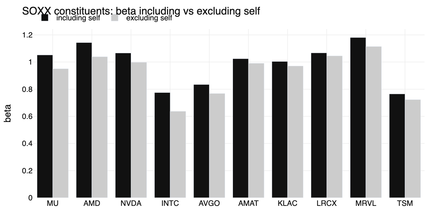
Everything about the calculation is held constant between the two versions — the only thing that changes is whether the stock sits inside or outside the benchmark it’s compared against. Any remaining difference is purely the mechanical effect.
Result
Run on the semiconductor sector (SOXX and its top-10 weighted constituents):
- Every single stock showed a positive self-weight effect (
beta_incl_self > beta_excl_self) — no exceptions. - Correlation of index weight with the size of the effect: 0.65 — heavier names get inflated more, exactly as the math predicts.
- This is a materially cleaner signal than the raw weight-vs-beta scatter, which only showed a correlation of 0.18 — because that comparison was also picking up noise from the benchmark’s other, non-synthetic holdings.
Why this matters for a model
If you’re training a cross-sectional model — ranking many stocks by predicted beta or predicted alpha — naive beta systematically biases those rankings toward heavily-weighted names, for reasons that have nothing to do with genuine predictive signal. Leave-one-out beta removes that bias and gives a fairer comparison across the universe.
Data quality caveat. The synthetic index here is built only from an ETF’s live top-10 holdings (the maximum Yahoo Finance exposes via its public fund-data endpoint) — not the true full index. Treat this as a demonstration of the mechanism, not an exact real-world beta figure. Live weights come from Ticker.funds_data.top_holdings; there is no free source for full, point-in-time historical index constituents, which is a genuine limitation for anyone trying to build a fully survivorship-bias-free backtest universe on a budget.