Labeling Financial Time Series for ML
Why the label matters more than the model
A model can only ever be as good as the question it was asked. Two researchers can use identical features and identical model architectures and end up with completely different, differently-useful systems purely because they defined the label — the “correct answer” the model trains against — differently. Changing a model’s architecture later is easy; realizing weeks in that the label asked the wrong question is expensive.
None of what follows is exotic. Every version below answers the same underlying question — “given today’s data, what happens next?” — but each answers it differently enough to produce a materially different model.
1. Direction — the simplest possible label
def label_direction(df, horizon=1):
    future_ret = df["close"].shift(-horizon) / df["close"] - 1
    return (future_ret > 0).astype(int)
Binary up/down, horizon bars ahead. Good first baseline — binary classification is easy to evaluate and debug — but it treats a +0.01% move and a +5% move identically.
2. A dead-band — ignore the moves that are just noise
def label_triple(df, horizon=5, thresh=0.005):
    fut = df["close"].shift(-horizon) / df["close"] - 1
    y = pd.Series(0, index=df.index)
    y[fut > thresh] = 1
    y[fut < -thresh] = -1
    return y
Tiny moves are mostly noise — trading on them costs fees and slippage for essentially no edge. Carving out an explicit “flat / no-trade” zone tends to produce a model whose confident predictions mean more, and a strategy that trades less for a similar or better edge.
3. Regression — predict the magnitude, not just the sign
def label_return(df, horizon=1):
    return df["close"].shift(-horizon) / df["close"] - 1
Richer than a classification label, since it captures how much, not just which way — useful if you want to size positions by predicted magnitude. Harder to fit well in practice, because the return distribution is heavily concentrated near zero, so a model can achieve deceptively low error by always predicting “close to zero.”
4. Volatility-adjusted — let the threshold flex with the instrument
def label_vol_adjusted(df, horizon=5, atr_col="atr_14", z_thresh=1.0):
    fut_ret = df["close"].shift(-horizon) / df["close"] - 1
    thresh = z_thresh * (df[atr_col] / df["close"])
    y = pd.Series(0, index=df.index)
    y[fut_ret > thresh] = 1
    y[fut_ret < -thresh] = -1
    return y
A fixed 0.5% threshold means something very different for a calm ETF than for a stock that regularly swings 3% a day. Scaling the threshold by each row’s own ATR keeps the label’s meaning roughly consistent — “an unusually large move for this instrument, right now” — across very different assets and volatility regimes.
5. Triple-barrier — the label that matches how you’d actually trade
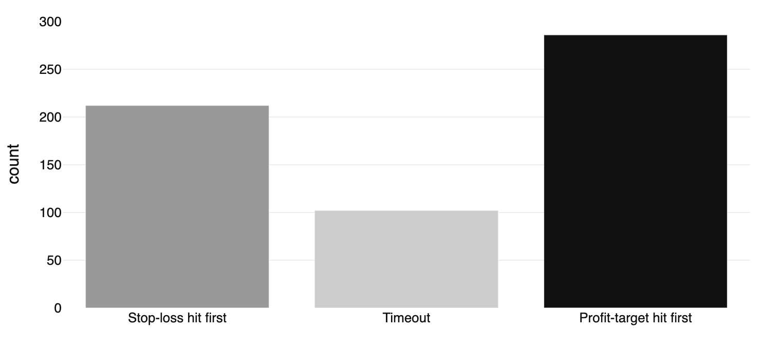
Every label above assumes you hold for exactly horizon bars no matter what happens along the way. Real trading doesn’t work like that: you’d take profit early, cut a loss early, or give up after a timeout. The triple-barrier method (López de Prado, Advances in Financial Machine Learning) labels each row by whichever of those three outcomes happens first.
def label_triple_barrier(df, horizon=20, pt_mult=2.0, sl_mult=2.0, atr_col="atr_14"):
    close, atr = df["close"].values, df[atr_col].values
    labels = np.zeros(len(df))

    for i in range(len(df) - horizon):
        entry = close[i]
        pt_level = entry + pt_mult * atr[i]     # profit-target barrier
        sl_level = entry - sl_mult * atr[i]      # stop-loss barrier
        window = close[i+1 : i+1+horizon]

        hit_pt = np.where(window >= pt_level)[0]
        hit_sl = np.where(window <= sl_level)[0]
        t_pt = hit_pt[0] if len(hit_pt) else np.inf
        t_sl = hit_sl[0] if len(hit_sl) else np.inf

        if t_pt < t_sl:   labels[i] = 1     # profit-target hit first
        elif t_sl < t_pt: labels[i] = -1    # stop-loss hit first
        # else: timeout, stays 0

    return pd.Series(labels, index=df.index)
A fixed-horizon label can call a trade “successful” even though price cratered through a stop-loss along the way and only happened to recover by the time the horizon elapsed — a trade you’d never actually have held to the end in real trading. Triple-barrier labels only ever encode outcomes that respect the risk management you’d actually use.
6. Meta-labeling — a second model that decides whether to trust the first
Once a directional model exists (any of the above), a second model can be layered on top whose only job is predicting “should I act on this signal?” — trained on whether the primary model’s calls turned out correct. This splits one hard problem into two easier ones: direction (primary model) and confidence (meta-model). In practice this is often where real gains come from — the primary model doesn’t need to improve at all; the meta-model just learns to filter out its low-conviction calls, typically improving the Sharpe ratio and win rate of what actually gets traded.
The trap that applies to all of the above: overlapping labels
Any label with horizon > 1 creates a subtle problem — the label at bar t and the label at bar t+1 share most of their look-ahead window. With horizon = 20, consecutive labels overlap in 19 of their 20 forward-looking bars: they are not independent observations, even though standard tooling (and metrics like accuracy) implicitly assumes every row is.
The practical risk: a dataset can look like it has thousands of independent training rows when the effective number of independent events is much smaller — one real price move can quietly influence dozens of overlapping labels, letting a model overfit to a handful of genuine events while appearing to have learned from a much larger sample.
Mitigations, roughly by effort: subsample non-overlapping rows (df.iloc[::horizon]); weight each sample’s loss contribution by how much its window overlaps its neighbors (“average uniqueness,” López de Prado); or, at minimum, make sure any walk-forward cross-validation gap is at least as wide as horizon — otherwise the validation set leaks into the training window’s label horizon.
Choosing a label
| Label | Captures | Main risk | Best for |
|---|---|---|---|
| Direction | up/down | noise near 50/50 | fast first baseline |
| Dead-band | up/down/flat | choosing the threshold | most classification work |
| Regression | full magnitude | tiny moves dominate the loss | sizing by confidence |
| Vol-adjusted | up/down/flat, instrument-relative | still fixed-horizon | multi-asset models |
| Triple-barrier | realistic trade outcome | needs uniqueness weighting | anything meant to mirror real execution |
| Meta-labeling | confidence in an existing signal | needs a working primary model first | improving an existing strategy’s Sharpe |